Detumbling Simulator

Detumbling Simulator is a MATLAB attitude-dynamics simulator for the pure magnetic detumbling of a fast-tumbling picosatellite: a spacecraft that leaves its deployer spinning at up to 180 °/s and must be brought to rest using nothing but three magnetorquers and two magnetometers, with no gyroscopes, no reaction wheels, and no attitude estimate. It closes the loop end to end (IGRF geomagnetic field, rigid-body dynamics, aerodynamic and residual-dipole disturbances, quantized and biased magnetometers, PWM-driven magnetorquers, and a B-dot control law with an autonomous detumbled/tumbling state machine) and wraps it in a Monte Carlo harness that disperses mass, inertia, actuator strength, and sensor errors across hundreds of runs. It is the simulator behind the IAC-18 paper Magnetic Detumbling of Fast-tumbling Picosatellites, developed for Delfi-PQ.

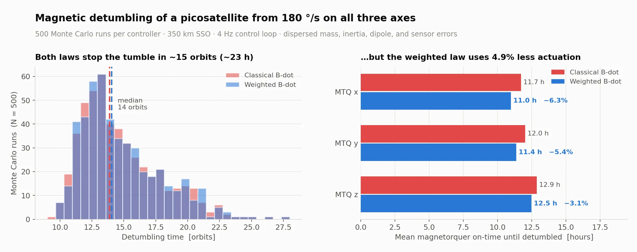
📊 The headline result, reproduced from the 500-run Monte Carlo campaigns committed in MC_Results/: the weighted B-dot law detumbles a 180 °/s tumble just as fast as the classical law, while keeping the magnetorquers energized 4.9 % less of the time.

Why This Simulator

• 🛰️ Sensor-realistic, not idealized: two magnetometers with independent noise, hard-iron bias, finite resolution (0.3 µT/LSb), and mounting rotations. The controller never sees the true field, only what a real BMX055 would report.
• 🧲 Actuator-realistic: magnetorquers are driven by a duty-cycled PWM signal with a finite rise time and a saturation limit, not by an ideal continuous dipole.
• 🔁 Autonomous state machine: a filtered tumble parameter decides when the satellite is detumbled and when it has started tumbling again, with hysteresis and confirmation timers, so the controller switches itself off and back on with no ground contact and no rate sensor.
• 🎲 Monte Carlo by construction: main(seed) returns a packed result column instead of plots, so hundreds of dispersed runs fan out over parfor; mass, inertia, maximum dipole, residual dipole, and sensor biases are all drawn from 3σ-truncated Gaussians.
• 🌍 Real environment models: IGRF-12 geomagnetic field, Keplerian LEO orbit with ECI/ECEF/BODY frame handling, aerodynamic torque from a six-face drag model, residual magnetic dipole, and gravity-gradient torque.
• ⏱️ Orbit caching: the expensive IGRF pass is computed once per orbit configuration and reused, turning subsequent runs from minutes into seconds.
• 📈 Reproducible results: the raw .mat data behind the paper's figures ships in MC_Results/, with the evaluation script that turns it into statistics and plots.

🔬 What "pure magnetic detumbling" means, and why it is hard

A magnetorquer can only produce a torque perpendicular to the local geomagnetic field, so at any instant the satellite is underactuated: the component of angular momentum along the field is uncontrollable. Detumbling works only because the field direction, as seen from the spinning body, keeps changing along the orbit. This makes the problem inherently slow (a full detumble takes ~15 orbits, roughly a day) and strongly dependent on orbit inclination.

The B-dot law exploits this by commanding a dipole opposing the measured rate of change of the field:

m_des = -k_w * d(b̂)/dt / ‖b‖

using the normalized field b̂, which makes the law insensitive to the field magnitude varying along the orbit. Crucially, d(b̂)/dt is computed by finite-differencing consecutive magnetometer samples, so no rate gyro and no attitude estimator are needed, which is exactly why B-dot is the standard choice for a picosatellite that has just been ejected and knows nothing about its own state.

The weighted B-dot law proposed in the paper scales the gain by the current tumble parameter, spending less actuation as the tumble decays, which is where the power saving in the figure above comes from.

Requirements

MATLAB R2018b or newer (the simulator uses vecnorm), plus these MathWorks toolboxes:

Toolbox	Needed for	Required to
Aerospace Toolbox	igrfmagm, decyear, ecef2lla, ned2ecefv	run any simulation
Parallel Computing Toolbox	parfor in run_mc.m	run a Monte Carlo campaign
Mapping Toolbox	load coast in the ground-track plot	render all plots in plots.m
Statistics and Machine Learning Toolbox	histfit, corr	run MC_Results/Eval_MC_results.m

Note

Only the Aerospace Toolbox is unavoidable: it supplies the IGRF geomagnetic field model at the heart of the environment. The other three gate optional stages (parallel campaigns, the ground-track plot, and MC post-processing), and the unit tests in tests/ deliberately run on bare MATLAB with no toolboxes at all.

No installation step is needed. Clone the repository and run from its root:

git clone https://github.com/rfonod/detumbling-simulator.git
cd detumbling-simulator

Quick Start

From the MATLAB prompt, with the repository root as the working directory:

main        % single deterministic run: simulates, then plots

That simulates 10 orbits (~4 h of orbital time) of a satellite tumbling at 30 °/s on all three axes, prints the orbit count as it goes, and opens the diagnostic figures: angular rates, quaternions, angular-momentum magnitude, true vs. measured magnetic field, B-dot, commanded magnetorquer duty cycles, the tumble parameter against its thresholds, and the ground track.

The first run of a new orbit configuration is slow (a few minutes) because the IGRF field is evaluated at every one of the ~44,000 time steps. The result is cached in Existing_Orbits/, and every later run with the same altitude, control frequency, and orbit count reuses it and takes seconds.

To watch a full detumble rather than a short excerpt, raise the tumble rate and the horizon at the top of main.m:

N_orb = 32;             % number of orbits to simulate
w0    = 180*[1;1;1]*d2r; % initial angular velocity: the paper's fast-tumbling case

Run the unit tests at any time (no toolboxes required):

runtests('tests')

Monte Carlo Campaigns

A single run tells you what happens to one satellite. The interesting question is what happens across the whole dispersion of build tolerances and sensor errors, which is what run_mc.m answers:

run_mc      % 500 dispersed runs over parfor; writes MC_Results/<out_name>.mat

Each worker calls main(seed, N_orb), which switches into Monte Carlo mode: it skips plotting, stops as soon as the satellite is detumbled, and returns one packed column of results. The dispersions applied per run are:

Parameter	Nominal	Dispersion (3σ-truncated Gaussian)
Mass	0.6 kg	±0.1 kg
Inertia (per axis)	from the geometry	±5 % on top of the mass uncertainty
Max. magnetic dipole (per axis)	0.002 A·m²	±15 %
Residual dipole	1e-4 A·m²	±10 % magnitude, random direction
Magnetometer bias	0.4 µT	random direction
Magnetometer noise	0.5 µT rms	redrawn every sample

Post-process a finished campaign with:

cd MC_Results
Eval_MC_results     % statistics, histograms, and parameter-correlation plots

Set ver, N_orb, C_type, and alt at the top of that script to pick a dataset, and cmp_act = 1 to load the companion controller and print the side-by-side comparison used in the paper.

📦 The packed result column

main in Monte Carlo mode returns a single column of 24 + 3*N_orb values, which run_mc.m assembles into a matrix and Eval_MC_results.m decodes:

Rows	Contents
1	t_det_w: true detumbling time, from the (unobservable) angular rate [s]
2	t_det_p: detumbling time as estimated by the algorithm from the tumble parameter [s]
3	Dispersed mass [kg]
4–6	Dispersed inertia, diag(I) [kg·m²]
7–9	Dispersed maximum dipole per axis [A·m²]
10–12	Dispersed residual dipole vector [A·m²]
13–15	Final tumble parameter [µT/s]
16–18	Initial angular velocity [rad/s]
19–21	Magnetorquer on-time per axis, up to t_det_w [s]
22–24	Magnetorquer on-time per axis, up to t_det_p [s]
25…	Magnetorquer on-time per axis, orbit by orbit (3 × N_orb values) [s]

A run that never detumbles within N_orb orbits leaves t_det_w as NaN; Eval_MC_results.m filters those columns out.

The gap between rows 1 and 2 is the quantity the state machine is judged on: how long after the satellite has actually stopped tumbling does the algorithm notice, using only magnetometer data. Across the committed campaigns it averages ~0.4 h, against a 1 h confirmation window.

How It Works

main.m is a single fixed-step loop running at the 4 Hz control frequency for N_orb orbits. Each iteration walks through the full chain:

1. Orbit: kepler2cart propagates a circular Keplerian LEO orbit (350 km, 96.85° inclination) to give position and velocity in ECI.
2. Environment: the state is rotated ECI → ECEF (rot_mat) → geodetic (ecef2lla), where igrfmagm evaluates the IGRF-12 geomagnetic field; the field is rotated back to ECI and into the body frame via the attitude quaternion (q2dcm).
3. Sensing: the true body-frame field is corrupted by each magnetometer's noise, bias, mounting rotation, and quantization, then fused into a weighted average.
4. Control: the normalized field is finite-differenced to get d(b̂)/dt, the B-dot law computes the desired dipole, and this is converted into a per-axis PWM on-time and sign, bounded by the duty cycle and the saturation limit.
5. State machine: the tumble parameter (a first-order filter of |d(b̂)/dt|) is compared against hysteresis thresholds; counters must stay satisfied for a full confirmation window before the controller declares the satellite detumbled and switches off, or tumbling and switches back on.
6. Dynamics: propag_att integrates the coupled quaternion kinematics and Euler equations (RK4 by default, sub-stepped to 0.125 s; ODE45 optional), driven by the magnetorquer torque, the residual-dipole torque, and the aerodynamic torque from dist_aer's six-face drag model.

All magnetic quantities are carried in µT through the ADCS path and converted to tesla only inside the propagator; every parameter line in main.m carries its unit in a trailing comment.

Configuration

Everything is configured by editing the parameter blocks at the top of main.m, each grouped by subsystem:

Block	Key parameters
Simulation	N_orb, q0, w0, no_C (no-control coast after release), att_solv (RK4 / ODE45), AirDens
Magnetorquers	m_x_max…m_z_max (saturation), m_rise, m_pol (polarity), m_res_mag (residual dipole)
Magnetometers	mag1_rms, mag1_res, mag1_bias_mag, mag1_S2B (mounting), w1/w2 (fusion weights)
Mass & geometry	mass, body and deployable-plate dimensions, from which the inertia tensor and drag areas are derived
Orbit	alt, inc, OMEGA, M0, Ldate (IGRF epoch)
Control algorithm	f_c (4 Hz), delta (duty cycle), alpha (tumble-parameter filter), p_bar_l/p_bar_u (hysteresis), t_bar_det/t_bar_tum (confirmation windows), k_w (B-dot gain)

The B-dot gain is not tuned by hand: it is derived from the orbit as k_w = 2·n·(1 + sin ξ_m)·min(I), following Avanzini & Giulietti, where n is the mean motion and ξ_m combines the orbit inclination with the geomagnetic tilt.

Repository Layout

Path	Contents
main.m	The simulator: parameters, environment, ADCS, and the simulation loop
propag_att.m	Attitude dynamics and kinematics, RK4 and ODE45 propagation
dist_aer.m	Aerodynamic disturbance torque (six-face drag model)
kepler2cart.m, q2dcm.m, rot_mat.m	Orbit and attitude conversion helpers
plots.m	Diagnostic figures for a single run
run_mc.m	Monte Carlo campaign driver
MC_Results/	Campaign data behind the paper, plus Eval_MC_results.m to analyze it
tests/	Unit tests for the kinematics and the propagator (bare MATLAB)
main_old.m, plots_old.m	v0.7 of the simulator, the version that produced the published results (see below)
Future/	v0.9 development line: solar radiation pressure, J2 gravity gradient, and the NRLMSISE-00 atmosphere

Important

Which file implements the paper's contribution? The weighted B-dot law, the paper's actual contribution and the source of the power saving in the figure above, lives in main_old.m, selected with C_type = 1 (C_type = 0 gives the classical law of Avanzini & Giulietti). The current main.m (v0.8) is a later refactor that carries a fixed B-dot gain and no C_type switch, so it reproduces the classical behaviour only. The datasets in MC_Results/ were generated with main_old.m. To reproduce the published weighted-law results, run main_old.m with C_type = 1.

Results

From the 500-run campaigns in MC_Results/ (350 km orbit, initial tumble of 180 °/s on all three axes, 32-orbit horizon):

Metric	Classical B-dot	Weighted B-dot
Detumbling time (mean)	14.8 orbits (22.5 h)	14.8 orbits (22.6 h)
Detumbling time (median)	13.9 orbits	14.0 orbits
Magnetorquer on-time, total	36.6 h	34.8 h (−4.9 %)
Magnetorquer on-time, x / y / z	11.7 / 12.0 / 12.9 h	11.0 / 11.4 / 12.5 h
Detection lag (algorithm vs. truth)	0.40 h	0.41 h

Detumbling performance is statistically indistinguishable between the two laws, while the weighted law keeps the magnetorquers off ~5 % longer, which matters on a picosatellite where the magnetorquers dominate the power budget during detumbling.

Limitations

• The orbit is circular and Keplerian: no J2 precession, no drag decay. Over the ~1 day of a detumble this is a reasonable approximation, but it is an approximation.
• The gravity-gradient torque is disabled in the torque sum: it is computed in main.m and handed to the propagator, but the line adding it is commented out in propag_att.m. The residual-dipole and aerodynamic torques are active.
• The default RK4 sub-step of 0.125 s is coarse at fast tumble rates. In torque-free motion at 180 °/s it loses about 2 % of the rotational kinetic energy over 25 s, an integrator truncation error that shrinks with the step size (see tests/test_dynamics.m). It is acceptable for the detumbling trend, which is what this simulator is for, but use att_solv = 'ODE45' for fidelity work at high rates.
• Air density is a fixed constant chosen from a three-level solar-activity table, not a dynamic atmosphere model. The Future/ line addresses this with NRLMSISE-00.
• Solar radiation pressure is not modelled in the main simulator.
• Parameters are edited in the source file; there is no configuration file or command-line interface.

Citing This Work

If you use Detumbling Simulator in your research, software, or product, please cite the following resources appropriately:

1. Preferred Citation: Please cite the associated conference paper for any use of the simulator, including research, applications, and derivative work:

   @InProceedings{fonod2018magnetic,
     author    = {Fonod, Robert and Gill, Eberhard},
     title     = {Magnetic Detumbling of Fast-tumbling Picosatellites},
     booktitle = {69th International Astronautical Congress},
     year      = {2018},
     month     = {October},
     address   = {Bremen, Germany},
     note      = {IAC-18-C1.3.11},
     url       = {https://research.tudelft.nl/files/47149549/IAC_18_C1_3_11_x46290.pdf}
   }

   Abstract: The problem of pure magnetic detumbling of a fast-tumbling picosatellite is considered. A new weighted B-dot control algorithm is proposed. The algorithm enables power reduction while not sacrificing detumbling performance. Analytical expressions relating the maximal expected rotational rate to the minimum sampling time required are presented. Simulation results demonstrate the practical benefits of the proposed approach for picosatellites.

2. Repository Citation: If you reference, modify, or build upon the software itself, please also cite the corresponding Zenodo release:

   @software{fonod2026detumbling,
     author  = {Fonod, Robert},
     license = {MIT},
     month   = jul,
     title   = {Detumbling Simulator: Magnetic Detumbling Control and Simulation for Fast-tumbling Picosatellites},
     url     = {https://github.com/rfonod/detumbling-simulator},
     doi     = {10.5281/zenodo.21346158},
     version = {1.0.0},
     year    = {2026}
   }

Each GitHub release is automatically archived to Zenodo; see CITATION.cff for the latest version and DOI.

Third-Party Code

This repository bundles three MATLAB File Exchange functions (putvar, truncatedGaussian, parfor_progress) and, in the Future/ line, the NRLMSISE-00 atmosphere model. Each remains the work of its author under its own terms. See THIRD_PARTY.md for the full attribution.

Contributing

Contributions are welcome. If you find a problem or have a suggestion, please open a GitHub Issue or submit a pull request.

License

This project is distributed under the MIT License. See the LICENSE file for details. Bundled third-party code retains its original license, as listed in THIRD_PARTY.md.